This Excel tutorial explains how to use the Excel LINEST function with syntax and examples.
x_values is the optional. It is the known set of "x values" from the line equation. If this parameter is omitted, x_values is assumed to be {1,2,3,...} with the same number of values as y_values.
constant is optional. It is either TRUE or FALSE. If this parameter is omitted, the function will assume TRUE. If constant is TRUE, b in the line equation is calculated normally. If constant is FALSE, b becomes 0 so that the line equation is evalulated as y = mx.
additional_statistics is optional. It is either TRUE or FALSE. If this parameter is omitted, the function will assume FALSE. If additional_statistics is TRUE, the function will return additional regression statistics. If additional_statistics is FALSE, the function will returns only m coefficients and b constant.
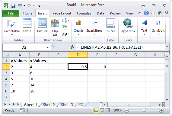
This first example we have entered the y values in column A (cells A2 through A6) and the x values in column B (cells B2 through B6). Then we have entered the following LINEST function in both cells D2 and E2 as follows:
The value in cell D2 returns the slope of 0.5 and the value in cell E2 returns the y-intercept of 0.
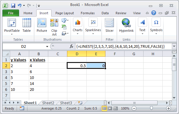
This formula could also be written as follows (entering values instead of cell ranges):

Description
The Microsoft Excel LINEST function uses the least squares method to calculate the statistics for a straight line and returns an array describing that line. The LINEST function uses the following line equation:y = mx + b (for a single range of x values) y = m1x1 + m2x2 + ... + b (for multiple ranges of x values)
Syntax
The syntax for the Microsoft Excel LINEST function is:LINEST( y_values, [x_values], [constant], [additional_statistics] )
Parameters or Arguments
y_values is the known set of "y values" from the line equation.x_values is the optional. It is the known set of "x values" from the line equation. If this parameter is omitted, x_values is assumed to be {1,2,3,...} with the same number of values as y_values.
constant is optional. It is either TRUE or FALSE. If this parameter is omitted, the function will assume TRUE. If constant is TRUE, b in the line equation is calculated normally. If constant is FALSE, b becomes 0 so that the line equation is evalulated as y = mx.
additional_statistics is optional. It is either TRUE or FALSE. If this parameter is omitted, the function will assume FALSE. If additional_statistics is TRUE, the function will return additional regression statistics. If additional_statistics is FALSE, the function will returns only m coefficients and b constant.
Applies To
The LINEST function can be used in the following versions of Microsoft Excel:- Excel 2013, Excel 2011 for Mac, Excel 2010, Excel 2007, Excel 2003, Excel XP, Excel 2000
Type of Excel Function
The LINEST function can be used in Microsoft Excel as the following type of function:- Worksheet function (WS)
Example (as Worksheet Function)
Let's look at some Excel LINEST function examples and explore how to use the LINEST function as a worksheet function in Microsoft Excel:This first example we have entered the y values in column A (cells A2 through A6) and the x values in column B (cells B2 through B6). Then we have entered the following LINEST function in both cells D2 and E2 as follows:
=LINEST(A2:A6,B2:B6,TRUE,FALSE)The LINEST functions are written as array formulas. When creating your array formula, you need to do the following:
- Enter the formulas in both cells D2 and E2
- Highlight cells D2 and E2
- Press F2 (in Windows) or CONTROL-U (on Mac)
- Press Ctrl+Shift+Enter
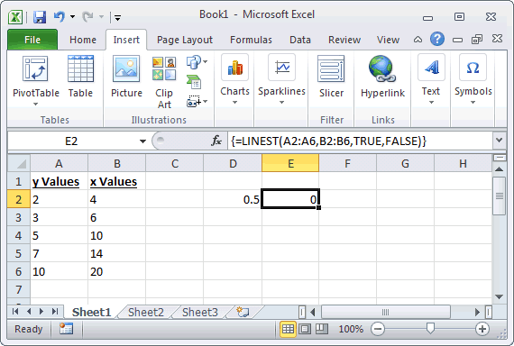
{=LINEST(A2:A6,B2:B6,TRUE,FALSE)}
You can see how the formula look in the images below.

The value in cell D2 returns the slope of 0.5 and the value in cell E2 returns the y-intercept of 0.
This formula could also be written as follows (entering values instead of cell ranges):
=LINEST({2,3,5,7,10},{4,6,10,14,20},TRUE,FALSE)
The LINEST functions are written as array formulas. When creating your array formula, you need to do the following:- Enter the formulas in both cells D2 and E2
- Highlight cells D2 and E2
- Press F2 (in Windows) or CONTROL-U (on Mac)
- Press Ctrl+Shift+Enter
{=LINEST({2,3,5,7,10},{4,6,10,14,20},TRUE,FALSE)}
